“Gapminder” Exploratory Data Analysis using R for Data Science

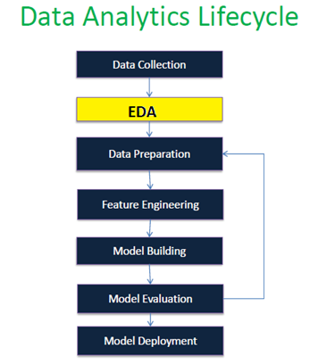
Main focus is to investigate the dataset Gapminder and interact with it. To illustrate the basic use of EDA in the dplyr,ggplot2 package, I use a “gapminder” datasets. This data is a data.frame created for the purpose of predicting sales volume.

• Using the dplyr package to perform data transformation and manipulation operations. 
• Using the ggplot2 package to visually analyze our data.

Load Packages

#install.packages("gapminder")
library(gapminder)
library(dplyr)
library(ggplot2)

The variables are explained as follows: Country — factor with 142 levels Continent — Factor with 5 levels Year — ranges from 1952 to 2007 in increments of 5 years lifeExp — life expectancy at birth, in years pop — population dgoPercap — GDP per capita

head(gapminder_unfiltered,5) #Unfiltered data

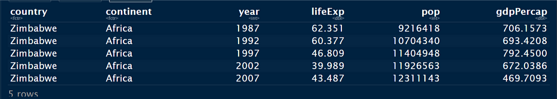
tail(gapminder_unfiltered,5)

Display name of Variables :

names(gapminder_unfiltered)

Data Cleaning :

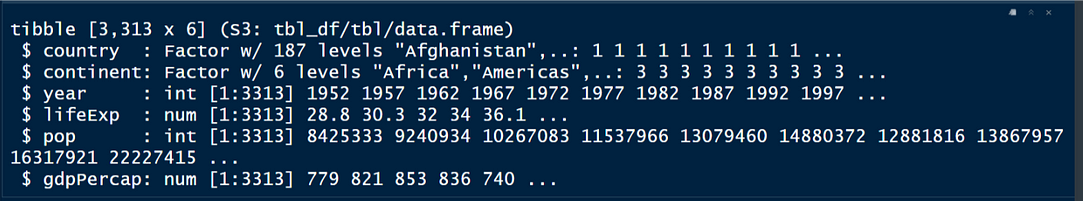
Finding the missing values as we can see this data has no missing values

str(gapminder_unfiltered)

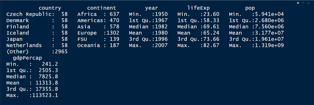
summary(gapminder_unfiltered) # see (Other) :2965

sum(is.na(gapminder_unfiltered))

[1] 0

Hence , we found zero NA values from this dataset .

Display the continent , country and year

unique(gapminder_unfiltered %>% select(year ,country, continent)) 

length(unique(gapminder_unfiltered$continent))

unique(gapminder_unfiltered$year)

Structure 

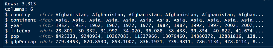
glimpse(gapminder_unfiltered)

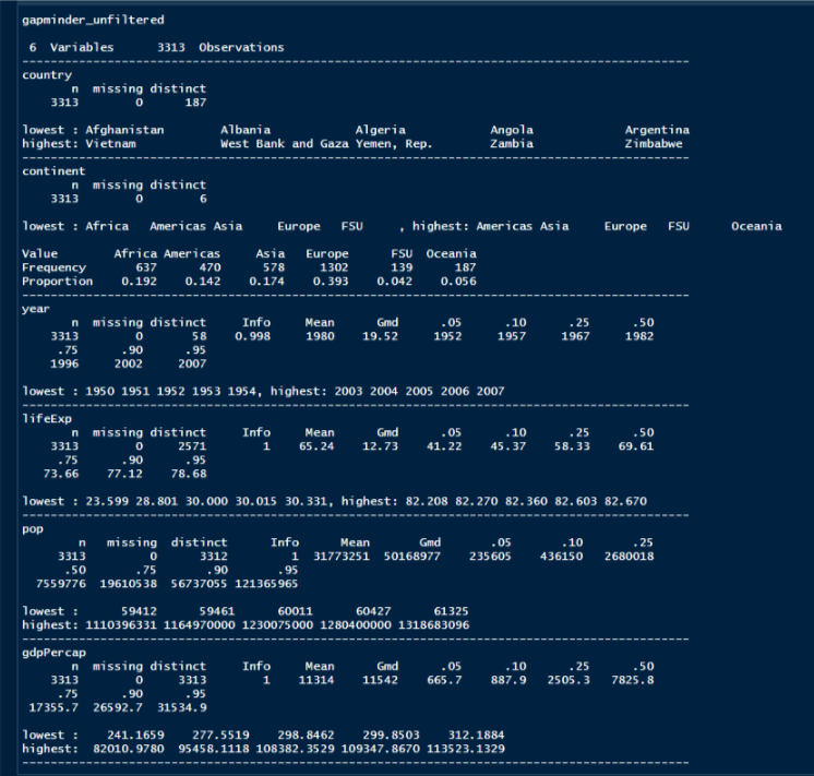
Summary Calculating descriptive statistics using describe()

Hmisc: Harrell Miscellaneous

Contains many functions useful for data analysis, high-level graphics, utility operations, functions for computing sample size and power, importing and annotating datasets, imputing missing values, advanced table making, variable clustering, character string manipulation, conversion of R objects to LaTeX and html code, and recoding variables.

library(Hmisc)
describe(gapminder_unfiltered)

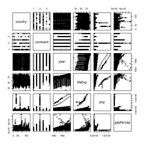
Exploratory Data Analysis

plot(gapminder_unfiltered) :

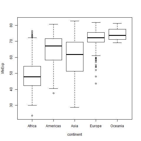
boxplot(lifeExp ~ continent) :

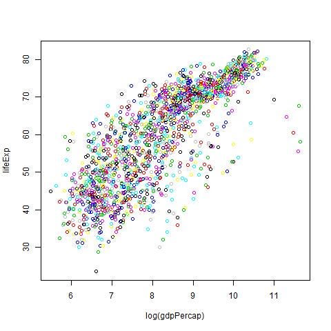
plot(lifeExp ~ log(gdpPercap),col = gdpPercap) :


For the year 2007, what is the distribution of GDP per capita across all countries?

GDP_2007 <- gapminder_unfiltered %>% filter(year == 2007)  %>% select(continent,country,gdpPercap)
GDP_2007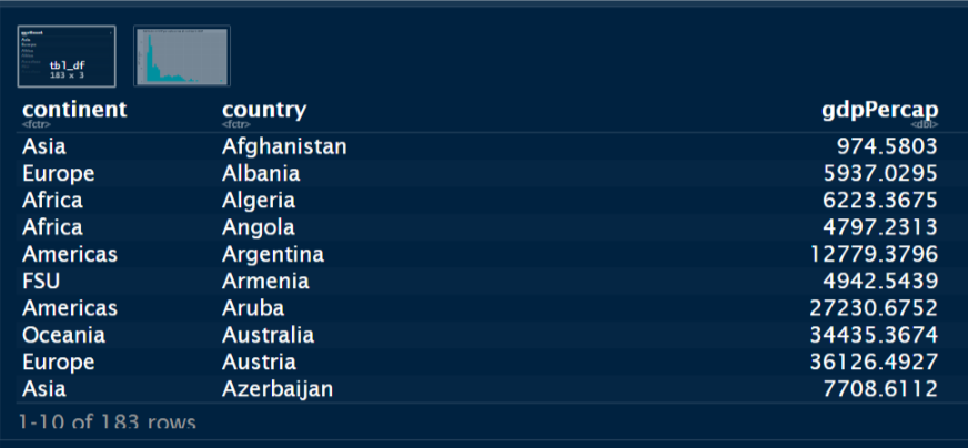 

ggplot(GDP_2007 ,aes(x =gdpPercap ))+geom_histogram( fill= "cyan" , 
bins = 40)+ ggtitle("Distribution of GDP per capita across all countries for 2007")+ylab("GDP per Capita")+
            theme(axis.title.x=element_blank(),
                  axis.text.x=element_blank(),
                  axis.ticks.x=element_blank())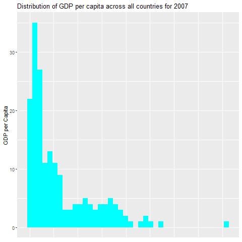

ggplot(GDP_2007, aes(x=country, y=gdpPercap)) +
 geom_point(aes(color = continent)) +
 ylab("GDP per Capita") +
 ggtitle("GDP Per Capita for Contries grouped by Continents for 2007")+
theme(axis.title.x=element_blank(),axis.text.x=element_blank(),axis.ticks.x=element_blank())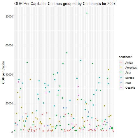 

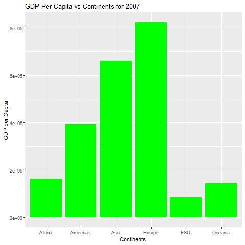
For the year 2007, how do the distributions differ across the different continents?

ggplot(GDP_2007, aes(x=continent, y=gdpPercap)) +geom_bar(fill = "green",stat = "identity") +
  xlab("Continents") +
  ylab("GDP per Capita") +
  ggtitle("GDP Per Capita vs Continents for 2007")

ggplot(GDP_2007, aes(continent,gdpPercap))+geom_jitter(aes(color = "fireebrick"))+
  xlab("Continents")+ylab("GDP per capita")+ggtitle("GDP per capital Vs Continents for 2007")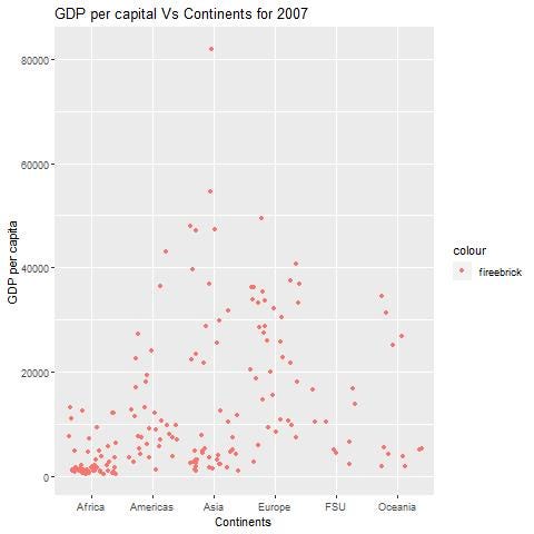

For the year 2007, what are the top 10 countries with the largest GDP per capita?

top_10_gdpc<- GDP_2007[order(GDP_2007$gdpPercap , decreasing = TRUE),2:3][1:10,] #,2:3 select col 2 to 3 only and show 1:10 entries 
top_10_gdpc

we can see the GDP per capita for specific country

GDP_2007[GDP_2007$country == "India",]

Top 10 GDP per capita by country

ggplot(top_10_gdpc, aes(x=country, y=gdpPercap)) +
  geom_bar(fill="palegreen2", stat = "identity") +
  xlab("Top 10 Countries") +ylab("GDP per Capita") +
  ggtitle("Top 10 GDP Per Capita vs Countries")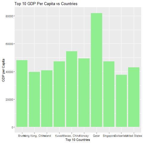 

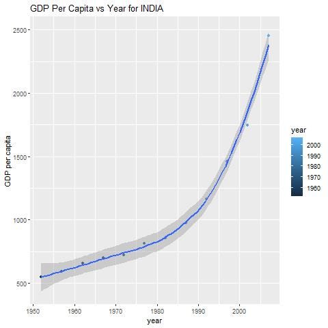
Plot the GDP per capita for your country of origin for all years available

GDP_India <- gapminder_unfiltered %>% filter(country == "India") %>%select(year,gdpPercap)
ggplot(GDP_India ,aes(year,gdpPercap , col =year ))+ geom_point()+geom_smooth()+ 
  xlab("year")+ylab("GDP per capita")+ggtitle("GDP Per Capita vs Year for INDIA")

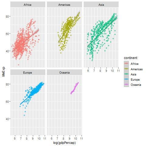
GDP per capita less than 50000 ,lifeExp and Continent

library(ggplot2)
gapminder %>% filter(gdpPercap < 50000 ) %>% ggplot(aes(log(gdpPercap),lifeExp,col = continent))+geom_point(alpha = 0.5)+geom_smooth(method = lm)+facet_wrap(~continent)

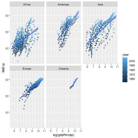
GPD per capita less than 50000 ,lifeExp and year

gapminder %>% filter(gdpPercap < 50000 ) %>% ggplot(aes(log(gdpPercap),lifeExp,col = year))+geom_point(alpha = 0.5)+geom_smooth(method = lm)+facet_wrap(~continent)

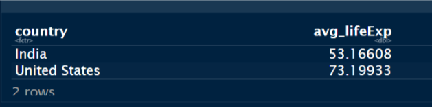
Life Expectancy of countries :

library(dplyr)
gapminder_unfiltered %>% 
  select(country , lifeExp) %>% filter(country == "United States" | country== "India" )%>% group_by( country) %>% summarise( avg_lifeExp = mean(lifeExp))

Check the life Expectancy using T test :

df1 <- gapminder_unfiltered %>% select(country , lifeExp) %>%filter(country == "United States" | country== "India" )  

t.test(data = df1 ,lifeExp ~ country )

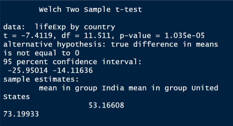
After Observing the “df” and “P value” there is significant difference in avg lifeExp of India and United States , so We reject the Null hypothesis here Pvalue is 5.311e-06.

---

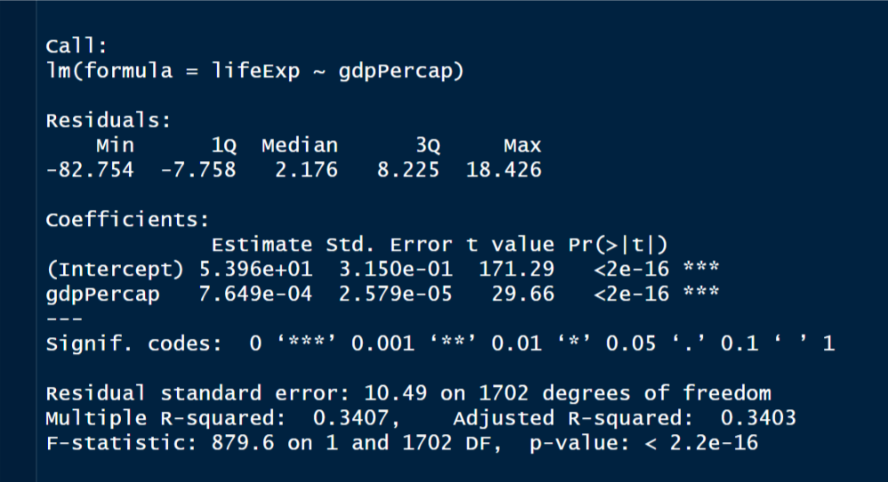
Bonus Information Just Introduction : ## Regression :

summary(lm(lifeExp ~ gdpPercap)) 

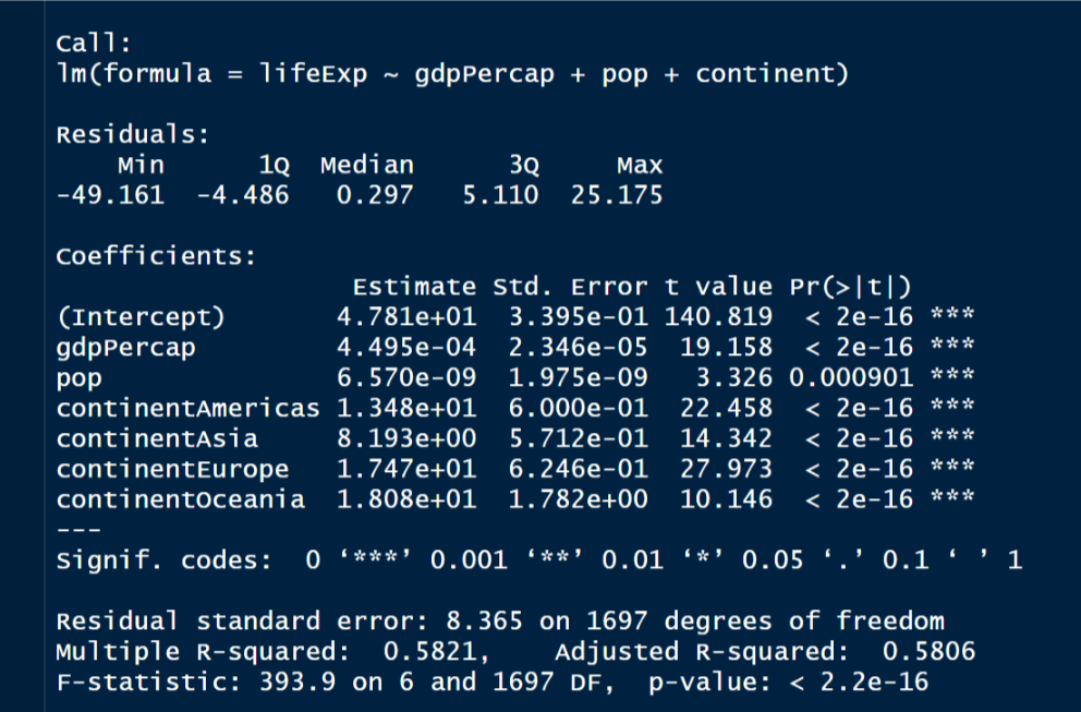
summary(lm(lifeExp ~ gdpPercap+pop+continent))

follow me on YouTube for Technical videos :

such simplified Data Science concepts will follow. If you liked this or have some feedback or follow-up questions please comment below. Thank you...